The Gram-Schmidt Process

The Gram-Schmidt process is s a simple algorithm for producing an orthogonal or orthonormal basis for any nonzero subspace of Rn.

Example: Let W = Span {x1, x2}, where x1 = [3, 6, 0] and x2 = [1, 2, 2]. Construct an orthogonal basis {v1, v2} for W.

The component of x2 is orthogonal to x1 is x2 - p, which is in W because it is formed from x2 and a  multiple of x1. Let v1=x1 and 

v2 = x2 - p = x2 - x2*x1/x1*x1 (*x1) = [1, 2, 2] - 15/45[3, 6, 0] = [0, 0,2].

Then {v1, v2} is an orthogonal basis set of nonzero vectors in W. Since dim W = 2, the set {v1, v2} is a basis for W. 

Theorem 11: The Gram-Schmidt Process: Given a basis {x1, ......., xp} for a nonzero subspace W of Rn, define 

v1=x1

v2 = x2 - x2*v1/v1*v1 *(v1)

v3 = x3 - x3*v1/v1*v1 *(v1) - x3*v2/v2*v2 *(v2)

vp = xp - xp*v1/v1*v1 *(v1) - xp*v2/v2*v2 *(v2) - xp*vp-1/vp-1*vp-1

Then {v1,....,vp} is an orthogonal basis for W. In addition Span {v1,....,vp} = Span{x1,....,xk} 

for 1< k<p.

Orthonormal  Bases: 

An orthonormal basis is constructed easily from an orthogonal basis {v1,.....vp}, simply normalize all the vk.

Example: In the first example we constructed the orthogonal basis v1 = [3, 6, 0] and v2 = [0, 0, 2] an orthogonal basis is 

u1= 1/||v|| (v1)= 1/sqrt(45) [3, 6, 0] = [1/sqrt(5), 2/sqrt(5), 0]

u2 = 1/||v|| (v2) = [0, 0, 1]

Fun Fact: QR Factorization of Matrices: 

if an m x n matrix A has linearly independent columns x1,....,xn then applying the Gram-Schmidt process (with normalizations) to x1,...., xn amounts to factoring A as described in the next theorem. This factorization is widely used in computer algorithms for various computations, such as solving equations. 

Theorem 12: The QR Factorization: If A is an m x n matrix with linearly independent columns, then A can be factored as A = QR, where Q is an m x n matrix whose columns form an orthonormal basis for ColA and R is an n x n upper triangular matrix with positive entries on its diagonal. 

Example: Find a QR factorization for A= [1, 0, 0]

                                                                   [1, 1, 0]

                                                                   [1, 1, 1]

                                                                   [1, 1, 1]

The columns of A are the vectors x1, x2 and x3. An orthogonal basis for Col A= Span{x1, x2, x3}. 

v1= [1, 1, 1, 1]

v2 = [-3, 1, 1, 1]

v3 = [0, -2/3, 1/3, 1/3]

To simplify the arithmetic, scale v3 by letting v'3 = 3v3. Then normalize the three vectors to obtain u1, u2, and u3 and use these vectors as the columns of Q: 

Q= [1/2, -3/sqrt(12), 0]

      [1/2, 1/sqrt(12), -2/sqrt(6)]

      [1/2, 1/sqrt(12), 1/sqrt(6)]

      [1/2, 1/sqrt(12), 1/sqrt(6)]

By construction, the first k columns of Q are an orthonormal basis of Span [x1,.....,xn}. From the proof of Theorem 12, A = QR for some R. To find R, observe that Q(transpose)Q = 1, because the columns of Q are orthonormal. Hence

Q(transpose)A= Q(transpose)(QR)= IR=R

R= [1/2, 1/2, 1/2, 1/2]

      [-3/sqrt(12), 1/sqrt(12), 1/sqrt(12), 1/sqrt(12)]

      [0, -2/sqrt(6), 1/sqrt(6), 1/sqrt(6)]

* A = [2, 3/2, 1]

          [ 0, 3/sqrt(12), 2/sqrt(12)]

          [0, 0, 2/sqrt(6)]

Examine Problems: 

1.) The columns of Q are obtained by applying the Gram-Schmidt process to the columns of A. Find an upper triangular matrix R such that A=QR. 

A(2, 4) matrix = [ 5, 9, 1, 5, -2, -4, 1, 5]

Q(2, 4) matrix = [-1, 6, 6, 3, -8, 3, 1, -2]

2.) The given set is a basis for a subspace of W. Use the Gram-Schmidt process to produce an orthogonal basis for W. 

[3, 0, 1], [8, 2, 5]

Inner Product, Length, and Orthogonality

*The Inner Product: if u and v are vectors in the real numbers, then we regard u and v as n x 1 matrices. The transpose u^T is a 1 x m matrix, and the matrix product u^Tv is a 1 x 1 matrix, which we write as a single real number (a scalar) without brackets. The number u^Tv is called the inner product of u and v, and often it is written as u*v. This inner product, is also known as the dot product. 

Example One: Compute u*v and v*u for u = [2, -5, -1] and v = [3,2,-3]. 

u*v = u^Tv =  (2)(3) + (-5)(2) + (-1)(-3) = (-1)

v*u = v^Tu = (3)(2) + (2)(-5) + 3)(-1) = (-1)

Theorem One: Let u, v and w be vectors in the real numbers, and let c be a scalar. Then

a.) u*v = v*u

b.) (u+v) *w = u*w + v*w

c.) (cu)*v = c(u*v) = u*(cv)

d.) u*u > or equal to 0, and u*u = 0 if and only if u = 0

*The length of a Vector: The length (or norm) of v is the non negative scalar //v// defined by 

//v// = sqrt (v*v) = sqrt (v1 + v2 +.....+ vn) and //v//^2 = v*v.

A vector whose length is 1 is called a unit vector. If we divide a nonzero vector v by its length - that is, multiply by 1/ //v// - we obtain a unit vector u because the length of us is (1/ //v//)//v//. The process creating u from v is sometimes called normalizing v, and we say that u is in the same direction as v. 

Example Two: Let v = (-1, -2, 2, 0). Find a unit vector u in the same direction as v. 

First compute the length of v: 

//v//^2 = v*v = (1)^2 + 2)^2 + (2)^2 +)^2 = 9

//v// = sqrt(9) = 3. 

Then, multiply v by 1/ //v// to obtain: 

u = 1/ //v// *v =1/3(v) =1/3 [1,-2,2,0] = [1/3, -2/3, 2/3, 0]

To check that //u// =1, it suffices to show that //u//^2 = 1. 

//u//^2 = u*u = (1/3)^2 + (2/3)^2 + (2/3)^2 + (0)^2

                     = 1/9 + 4/9 + 4/9 + 0 =1

For u and v in real numbers, the distance between u and v, written as dist(u,v), is the length of the vector u-v. That is, dist(u,v) = //u-v//.

Two vectors u and v in the real numbers are orthogonal to each other if u*v = 0.

Theorem Two: The Pythagorean Theorem: 

Two vectors u and v are orthogonal if and only if //u+v//^2 = //u//^2 + //v//^2.

If a vector z is orthogonal to every vector in a subspace W of all the real numbers, then z is said to be orthogonal to W. The set of all vectors z that are orthogonal to W is called the orthogonal component of W and is denoted by W (perp). 

Theorem Three: Let A be an m x n matrix. The orthogonal complement of the row space of A is the null space of A, and the orthogonal complement of the column space of A is the null space of A transpose: (Row A) (perp) = Nul A and (Col A) (perp) = Nul A transpose. 

If u and v are nonzero vectors in either R^2 or R^3, then there is a nice connection between their inner product and the angle theta between the two line segments from the origin to the points identified with u and v. The formula is u*v = //u// //v// cos (theta).

Examine Problem: 

Mark each statement True of False and Justify your answer. 

a.) v*v = //v//^2

b.) For any scalar c, u*(cv) = c(u*v)

c.) If the distance from u to v equals the distance from u to -v, then u and v are orthogonal. 

d.)For a square matrix A, vectors in Col A are orthogonal to vectors in Nul A. 

e.) For an m x n matrix A vectors, in the null space of A are orthogonal to vectors in the row space of A. 

Applications to Markov Chains

The Markov chains described in this section are used as mathematical models of a wide variety of situations in biology, business, chemistry, engineering, physics, and elsewhere. In each case, the model is used to describe an experiment or measurement that is preformed many times in the same way, where the outcome of the trial of the experiment will be one of several specified possible outcomes, and where the outcome of one trial depends only on the immediately preceding trial.

A vector with nonnegative entries that add up to 1 is called a probability vector. A stochastic matrix is a square matrix whose columns are probability vectors. A Markov chain is a sequence of probability vectors x0, x1, x2,.... together with a stochastic matrix P, such that x1=Px0, x2=Px1....Then the Markov chain described by the first order difference equation xi+1=Pxk for k=0,1,2.....

When a Markov chain of vectors in R^n describes a system or a sequence of experiments, the entries in xk, the probabilities that the system is in each of n possible states, or the probabilities that the outcome of the experiment is one of n possible outcomes. For this reason, xk is often called a state vector.

Example One: Examine a model for population movement between a city and its suburbs. The annual migration between these two parts of the metropolitan region was governed by the migration matrix M.

From: 

City Suburbs      

M = [.95        .03 ]                

[.05        .97 ]       

That is each year 5% of the population moved to the suburbs, and 3% of the suburban population moves to the city. The columns of M are probability vectors, so M is a stochastic matrix. Suppose the 2014 population of the region is 600,000 in the city and 400,000 in the suburbs. Then the initial distribution population in the region is given by x0. What is the distribution population in 2015? in 2016? 

After one year, the population vector 

[600,000

400,000]

changed to 

[.95    .03  x  600,000] = [582,000]

[.05    .97  x  400,000] = [418,000]

If we divide by both sides of the this equation by the total population of 1 million, and use the fact that kMx= M(kx), we find that 

[.95  .03  x .600 = [.582]

[.05  .97  x .400 = [.418]

The vector x1 = [.582

                           .418]

gives the population distribution in 2015. that is 58.2% of the region lived in the city and 41.8% lived in the suburbs. Similarly the population distribution in 2016 is described by a vector x2, where

x2 = Mx1 = [.95  .03  x  .582] = [.565]

                     [.05  .97  x .418]   =[.435]

gives the population distribution in 2016, that is 56.5% of the region lived in the city and 43.5% lived in the suburbs. 

If P is a stochastic matrix, then the steady-state vector (or equilibrium vector) for P is a probability vector q such that pq=q it can be shown that every stochastic matrix has a steady-state vector. 

Example two: The probability vector q = [.375

                                                               .625] is a steady state vector for the population migration matrix M, because 

Mq = [.95  .03  x  .375] = [.35625 + .01875] = [.375] q

          [.05  .97  x  .625] = [.01875 + .60625] = [.625] q

If the total populaiton in example one, is 1 million, then q in this example would correspond to having 375,000 persons in the city and 625,000 in the suburbs. At the end of one year, the migration out of the city would be (.05)(375,000) = 18,750 persons, and the migration into the city from the suburbs would be (0.3)(625,000) = 18,750 persons. As a result, the populaiton in the city would remain the same. Similarly, the suburban populaiton would be stable. 

Theorem 18: If P is an mxn regular stochastic matrix, then P has a unique steady-state vector q. Further, xo is any initial state and xk+1 = Pxk, for k = 0,1,2,....then the Markov chain {xk} converges to q as k goes to infinity. 

Examine Problem: On any given day a student is either healthy or ill. Of the students who are healthy today, 95% will be healthy tomorrow. Of the students who are ill today, 55% will still be ill tomorrow. 

a.) What is the stochastic matrix for this situation?

b.) Suppose 20% of the students are ill on Monday. What faction or percentage of the students are likely to be ill on Tuesday or Wednesday? 

c.) If a student is well today, what is the probability that he or she will be well two days from now? 

Solving matrixes using cofactor expansion:

Co-factor Expansion: 

Formula: Given A= [aij], the (i, j) cofactor of A is the number Cij given by Cij=(-1)^(i+j) det Aij

then det A= a11C11+a12C12+......+a1nC1n. This formula is called a cofactor expansion across the first row of A. 

Theorem One: The determinant of an m x n matrix A can by computed by a cofactor expansion across any row or down any column. The expansion across the ith row using the cofactors in the above equation is det A = a11C11+a12C12+....+a1nC1n. The cofactor expansion down the jth column is det A= a1jC1j+a2jC2j+.....+anjCnj. 

The plus or minus sign is the (i,j)-cofactor depends on the position of a1j in the matrix, regardless of the sign of a1j itself. The factor (-1)^(i+j) determines the following checkerboard pattern of signs: 

Example One: Use a cofactor expansion to solve the matrix. 

Theorem One is helpful for computing the determinant of a matrix that contains many zeros. For example, if a row is mostly zeros, then the cofactor expansion across that row has many terms that are zero, and the cofactors in those terms need not to be calculated. The same approach works with a column that contains many zeros. 

Examples: Find the cofactor expansion for each matrix. 

Theorem Two: If A is a triangular matrix, then det A is the product of the entries on the main diagonal of A. 

Example: Find the cofactor expansion

Note: Today's standards, a 25 x 25 matrix is small. Yet it would be impossible to calculate a 25 x 25 determinant by cofactor expansion. In general, a cofactor expansion requires more than n! multiplications, and 25! is approximately 1.5 x 10^25. If a computer performs one trillion multiplications per second, it would have to run for more than 500,000 years to compute a 25 x 25 determinant by this method. 

Examine Problem: Find the cofactor expansion and the determinant of the following matrix equation.

Linear Algebra 2- Properties of Matrix Multiplication (2.1)

Matrix Multiplication: 
Theorem 2: Let A be an m x m matrix, and let B and C have sizes for which the indicated sums and products are defined.
a.) A(BC) = (AB)C                                                (Associative Law of Multiplication)
corresponds to composition of linear transformations.
b.) A(B+C) = AB+AC                                           (Left Distributive Law)
c.) (B+C)A = BA+CA                                           (Right Distributive Law)
d.) r(AB) = (rA)B = A(rB)
for any scalar r.
e.) I_mA = A = AI_m                                             (Identity for Matrix Multiplication)

Example: Product 

Example: Associative Law of Multiplication: 

Example: Identity for Matrix Multiplication:

Warnings: 
1. In general, AB does not equal BA.
2. The cancellation laws do not fold for matrix multiplication. that is, if AB = AC, then it is not true in general that B = C.
3. If a product AB is the zero matrix, you cannot conclude in general that either A = 0 or B = 0.

Powers of a Matrix: 
If A is an n x n matrix and if k is a positive integer, then A^k denotes the product of k copies of A.
                                                    A^k = A x A x A.....
If A is nonzero and if x is in R^n, then A^k is the result of left multiplying x by A in the amount of k times. If k = 0 then A^0x should be x itself, which will be the identity matrix.

Example: 

 











Example: 

If you still need some help with matrix multiplication here is a good link to help you out.
https://www.mathsisfun.com/algebra/matrix-multiplying.html
Also i have found a really good video on Powers of a Matrix and how to use the powers as an implication of multiply matrix's. Its called power of Matrix's and you can find it on Youtube.

An example problem could be: Find all properties from theorem 2 (a-e) and also find the power matrix's for A, B, and C.

Solving One-Variable Linear Equations

Solving One Variable Equations: 

"Linear equations are equations with a plain old variable like "x" rather than something more complicated like "x^2"

You've probably already solved linear equations; you just didn't know it. 

When solving a one variable equation, you need to "undo" whatever has been done to the variable. 

 A solution: a solution to an equation is a value or set of values that makes the equation true. 

For Example in the Equation: 

x + 2 = 3

the solution is x = 1, because 1 + 2 = 3. 

Lets Review: Additive Inverse: 

An additive number is something you add to a number to make it equal 0. 

2 + (-2) = 0

5 + -5 = 0

Multiplicative Inverse: 

A multiplicative inverse is something you multiple by another number to equal 1. 

2 X 1/2 = 1

You do this in order to get the variable by itself; in technical terms you are "isolating the variable."

For Example: x + 6 = -3

You first want to get the x on the left side by itself. So you will subtract the 6 to the right side. So now the equation looks like x = -3 - 6. So now we solve for x. -3 - 6 = -9. So x = -9.

Whatever you do to an equation,
do the   S A M E   thing
to   B O T H   sides of that equation!

Example: x - 3 = -5

Since you want to get x by itself, so you want to add 3 to both sides. 

x - 3 = -5

+3 = +3 

x = -2

Then the solution is x = -2. 

Lets solve this equation: 3x + 6 + 4x = 13

First we need to combine like terms: those terms are the 3x + 4x = 7x. 

So now the equation look like this: 7x + 6 = 13

So now to get the variable by itself we need to subtract the 6 from both sides. 

So we get 7x = 13 - 6

7x = 7

now we divide by 7 to get x by itself to both sides. 

So x = 1. 

Now we need to check our work

3 (1) + 6 + 4 (1) = 13

3 + 6 + 4 = 13

13 = 13. 

Therefore the solution is x = 1. 

Lets solve this equation: 3 - 5x = 18.

First we need to move the 3 to the other side to get x by itself, so lets subtract the 3 from both sides.

-5x = 18 - 3

-5x = 15. 

Now we need to divide by the -5 to get x by itself. 

x = 15 / -5

x = -3.

Now we need to check our work so we plug x = -3 back into the equation. 

3 - 5(-3) = 18

3 - (-15) = 18

18 = 18. 

Therefore the solution is x = -3. 

Oder of Operations

Order of Operations: 

What is the answer to this ? 4 + 6 x 2 =

Did you get 20?

Can you see how the answer could be 16?

There are two possible ways to figure out this problem. 

          Do the addition first :                                                 Do the multiplication first: 

                4 + 6 x 2 =                                                                                  4 + 6 x 2 =

                    10 x 2 =20                                                                                  4 + 12 = 16

Which is it? 

Both answers can't be right or we would always be arguing to the answers of math problems. The nice thing about math is there is always just ONE answer. 

So a long time ago mathematicians decided to make a set of rules for what to do first in a math problem. 

The rules are called the Order of Operations!

which is abbreviated by PEMDAS.

The P in PEMDAS stands for "parenthesis"

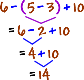
Parenthesis in math are used to group important things together, so you always do them first. 

For example: 

 Do inside the parenthesis first:

Here's another Example: 

 In this problem we have to do paranthesis first then exponents then division.

The classic sentence that math geeks have been using for years to remember the Order of Operations (PEMDAS) is: 

Please Excuse My Dear Aunt Sally

Can you think of a sentence to go along with this acronym?