The Gram-Schmidt Process

The Gram-Schmidt process is s a simple algorithm for producing an orthogonal or orthonormal basis for any nonzero subspace of Rn.

Example: Let W = Span {x1, x2}, where x1 = [3, 6, 0] and x2 = [1, 2, 2]. Construct an orthogonal basis {v1, v2} for W.

The component of x2 is orthogonal to x1 is x2 - p, which is in W because it is formed from x2 and a  multiple of x1. Let v1=x1 and 

v2 = x2 - p = x2 - x2*x1/x1*x1 (*x1) = [1, 2, 2] - 15/45[3, 6, 0] = [0, 0,2].

Then {v1, v2} is an orthogonal basis set of nonzero vectors in W. Since dim W = 2, the set {v1, v2} is a basis for W. 

Theorem 11: The Gram-Schmidt Process: Given a basis {x1, ......., xp} for a nonzero subspace W of Rn, define 

v1=x1

v2 = x2 - x2*v1/v1*v1 *(v1)

v3 = x3 - x3*v1/v1*v1 *(v1) - x3*v2/v2*v2 *(v2)

vp = xp - xp*v1/v1*v1 *(v1) - xp*v2/v2*v2 *(v2) - xp*vp-1/vp-1*vp-1

Then {v1,....,vp} is an orthogonal basis for W. In addition Span {v1,....,vp} = Span{x1,....,xk} 

for 1< k<p.

Orthonormal  Bases: 

An orthonormal basis is constructed easily from an orthogonal basis {v1,.....vp}, simply normalize all the vk.

Example: In the first example we constructed the orthogonal basis v1 = [3, 6, 0] and v2 = [0, 0, 2] an orthogonal basis is 

u1= 1/||v|| (v1)= 1/sqrt(45) [3, 6, 0] = [1/sqrt(5), 2/sqrt(5), 0]

u2 = 1/||v|| (v2) = [0, 0, 1]

Fun Fact: QR Factorization of Matrices: 

if an m x n matrix A has linearly independent columns x1,....,xn then applying the Gram-Schmidt process (with normalizations) to x1,...., xn amounts to factoring A as described in the next theorem. This factorization is widely used in computer algorithms for various computations, such as solving equations. 

Theorem 12: The QR Factorization: If A is an m x n matrix with linearly independent columns, then A can be factored as A = QR, where Q is an m x n matrix whose columns form an orthonormal basis for ColA and R is an n x n upper triangular matrix with positive entries on its diagonal. 

Example: Find a QR factorization for A= [1, 0, 0]

                                                                   [1, 1, 0]

                                                                   [1, 1, 1]

                                                                   [1, 1, 1]

The columns of A are the vectors x1, x2 and x3. An orthogonal basis for Col A= Span{x1, x2, x3}. 

v1= [1, 1, 1, 1]

v2 = [-3, 1, 1, 1]

v3 = [0, -2/3, 1/3, 1/3]

To simplify the arithmetic, scale v3 by letting v'3 = 3v3. Then normalize the three vectors to obtain u1, u2, and u3 and use these vectors as the columns of Q: 

Q= [1/2, -3/sqrt(12), 0]

      [1/2, 1/sqrt(12), -2/sqrt(6)]

      [1/2, 1/sqrt(12), 1/sqrt(6)]

      [1/2, 1/sqrt(12), 1/sqrt(6)]

By construction, the first k columns of Q are an orthonormal basis of Span [x1,.....,xn}. From the proof of Theorem 12, A = QR for some R. To find R, observe that Q(transpose)Q = 1, because the columns of Q are orthonormal. Hence

Q(transpose)A= Q(transpose)(QR)= IR=R

R= [1/2, 1/2, 1/2, 1/2]

      [-3/sqrt(12), 1/sqrt(12), 1/sqrt(12), 1/sqrt(12)]

      [0, -2/sqrt(6), 1/sqrt(6), 1/sqrt(6)]

* A = [2, 3/2, 1]

          [ 0, 3/sqrt(12), 2/sqrt(12)]

          [0, 0, 2/sqrt(6)]

Examine Problems: 

1.) The columns of Q are obtained by applying the Gram-Schmidt process to the columns of A. Find an upper triangular matrix R such that A=QR. 

A(2, 4) matrix = [ 5, 9, 1, 5, -2, -4, 1, 5]

Q(2, 4) matrix = [-1, 6, 6, 3, -8, 3, 1, -2]

2.) The given set is a basis for a subspace of W. Use the Gram-Schmidt process to produce an orthogonal basis for W. 

[3, 0, 1], [8, 2, 5]

Inner Product, Length, and Orthogonality

*The Inner Product: if u and v are vectors in the real numbers, then we regard u and v as n x 1 matrices. The transpose u^T is a 1 x m matrix, and the matrix product u^Tv is a 1 x 1 matrix, which we write as a single real number (a scalar) without brackets. The number u^Tv is called the inner product of u and v, and often it is written as u*v. This inner product, is also known as the dot product. 

Example One: Compute u*v and v*u for u = [2, -5, -1] and v = [3,2,-3]. 

u*v = u^Tv =  (2)(3) + (-5)(2) + (-1)(-3) = (-1)

v*u = v^Tu = (3)(2) + (2)(-5) + 3)(-1) = (-1)

Theorem One: Let u, v and w be vectors in the real numbers, and let c be a scalar. Then

a.) u*v = v*u

b.) (u+v) *w = u*w + v*w

c.) (cu)*v = c(u*v) = u*(cv)

d.) u*u > or equal to 0, and u*u = 0 if and only if u = 0

*The length of a Vector: The length (or norm) of v is the non negative scalar //v// defined by 

//v// = sqrt (v*v) = sqrt (v1 + v2 +.....+ vn) and //v//^2 = v*v.

A vector whose length is 1 is called a unit vector. If we divide a nonzero vector v by its length - that is, multiply by 1/ //v// - we obtain a unit vector u because the length of us is (1/ //v//)//v//. The process creating u from v is sometimes called normalizing v, and we say that u is in the same direction as v. 

Example Two: Let v = (-1, -2, 2, 0). Find a unit vector u in the same direction as v. 

First compute the length of v: 

//v//^2 = v*v = (1)^2 + 2)^2 + (2)^2 +)^2 = 9

//v// = sqrt(9) = 3. 

Then, multiply v by 1/ //v// to obtain: 

u = 1/ //v// *v =1/3(v) =1/3 [1,-2,2,0] = [1/3, -2/3, 2/3, 0]

To check that //u// =1, it suffices to show that //u//^2 = 1. 

//u//^2 = u*u = (1/3)^2 + (2/3)^2 + (2/3)^2 + (0)^2

                     = 1/9 + 4/9 + 4/9 + 0 =1

For u and v in real numbers, the distance between u and v, written as dist(u,v), is the length of the vector u-v. That is, dist(u,v) = //u-v//.

Two vectors u and v in the real numbers are orthogonal to each other if u*v = 0.

Theorem Two: The Pythagorean Theorem: 

Two vectors u and v are orthogonal if and only if //u+v//^2 = //u//^2 + //v//^2.

If a vector z is orthogonal to every vector in a subspace W of all the real numbers, then z is said to be orthogonal to W. The set of all vectors z that are orthogonal to W is called the orthogonal component of W and is denoted by W (perp). 

Theorem Three: Let A be an m x n matrix. The orthogonal complement of the row space of A is the null space of A, and the orthogonal complement of the column space of A is the null space of A transpose: (Row A) (perp) = Nul A and (Col A) (perp) = Nul A transpose. 

If u and v are nonzero vectors in either R^2 or R^3, then there is a nice connection between their inner product and the angle theta between the two line segments from the origin to the points identified with u and v. The formula is u*v = //u// //v// cos (theta).

Examine Problem: 

Mark each statement True of False and Justify your answer. 

a.) v*v = //v//^2

b.) For any scalar c, u*(cv) = c(u*v)

c.) If the distance from u to v equals the distance from u to -v, then u and v are orthogonal. 

d.)For a square matrix A, vectors in Col A are orthogonal to vectors in Nul A. 

e.) For an m x n matrix A vectors, in the null space of A are orthogonal to vectors in the row space of A. 

Applications to Markov Chains

The Markov chains described in this section are used as mathematical models of a wide variety of situations in biology, business, chemistry, engineering, physics, and elsewhere. In each case, the model is used to describe an experiment or measurement that is preformed many times in the same way, where the outcome of the trial of the experiment will be one of several specified possible outcomes, and where the outcome of one trial depends only on the immediately preceding trial.

A vector with nonnegative entries that add up to 1 is called a probability vector. A stochastic matrix is a square matrix whose columns are probability vectors. A Markov chain is a sequence of probability vectors x0, x1, x2,.... together with a stochastic matrix P, such that x1=Px0, x2=Px1....Then the Markov chain described by the first order difference equation xi+1=Pxk for k=0,1,2.....

When a Markov chain of vectors in R^n describes a system or a sequence of experiments, the entries in xk, the probabilities that the system is in each of n possible states, or the probabilities that the outcome of the experiment is one of n possible outcomes. For this reason, xk is often called a state vector.

Example One: Examine a model for population movement between a city and its suburbs. The annual migration between these two parts of the metropolitan region was governed by the migration matrix M.

From: 

City Suburbs      

M = [.95        .03 ]                

[.05        .97 ]       

That is each year 5% of the population moved to the suburbs, and 3% of the suburban population moves to the city. The columns of M are probability vectors, so M is a stochastic matrix. Suppose the 2014 population of the region is 600,000 in the city and 400,000 in the suburbs. Then the initial distribution population in the region is given by x0. What is the distribution population in 2015? in 2016? 

After one year, the population vector 

[600,000

400,000]

changed to 

[.95    .03  x  600,000] = [582,000]

[.05    .97  x  400,000] = [418,000]

If we divide by both sides of the this equation by the total population of 1 million, and use the fact that kMx= M(kx), we find that 

[.95  .03  x .600 = [.582]

[.05  .97  x .400 = [.418]

The vector x1 = [.582

                           .418]

gives the population distribution in 2015. that is 58.2% of the region lived in the city and 41.8% lived in the suburbs. Similarly the population distribution in 2016 is described by a vector x2, where

x2 = Mx1 = [.95  .03  x  .582] = [.565]

                     [.05  .97  x .418]   =[.435]

gives the population distribution in 2016, that is 56.5% of the region lived in the city and 43.5% lived in the suburbs. 

If P is a stochastic matrix, then the steady-state vector (or equilibrium vector) for P is a probability vector q such that pq=q it can be shown that every stochastic matrix has a steady-state vector. 

Example two: The probability vector q = [.375

                                                               .625] is a steady state vector for the population migration matrix M, because 

Mq = [.95  .03  x  .375] = [.35625 + .01875] = [.375] q

          [.05  .97  x  .625] = [.01875 + .60625] = [.625] q

If the total populaiton in example one, is 1 million, then q in this example would correspond to having 375,000 persons in the city and 625,000 in the suburbs. At the end of one year, the migration out of the city would be (.05)(375,000) = 18,750 persons, and the migration into the city from the suburbs would be (0.3)(625,000) = 18,750 persons. As a result, the populaiton in the city would remain the same. Similarly, the suburban populaiton would be stable. 

Theorem 18: If P is an mxn regular stochastic matrix, then P has a unique steady-state vector q. Further, xo is any initial state and xk+1 = Pxk, for k = 0,1,2,....then the Markov chain {xk} converges to q as k goes to infinity. 

Examine Problem: On any given day a student is either healthy or ill. Of the students who are healthy today, 95% will be healthy tomorrow. Of the students who are ill today, 55% will still be ill tomorrow. 

a.) What is the stochastic matrix for this situation?

b.) Suppose 20% of the students are ill on Monday. What faction or percentage of the students are likely to be ill on Tuesday or Wednesday? 

c.) If a student is well today, what is the probability that he or she will be well two days from now? 

Solving matrixes using cofactor expansion:

Co-factor Expansion: 

Formula: Given A= [aij], the (i, j) cofactor of A is the number Cij given by Cij=(-1)^(i+j) det Aij

then det A= a11C11+a12C12+......+a1nC1n. This formula is called a cofactor expansion across the first row of A. 

Theorem One: The determinant of an m x n matrix A can by computed by a cofactor expansion across any row or down any column. The expansion across the ith row using the cofactors in the above equation is det A = a11C11+a12C12+....+a1nC1n. The cofactor expansion down the jth column is det A= a1jC1j+a2jC2j+.....+anjCnj. 

The plus or minus sign is the (i,j)-cofactor depends on the position of a1j in the matrix, regardless of the sign of a1j itself. The factor (-1)^(i+j) determines the following checkerboard pattern of signs: 

Example One: Use a cofactor expansion to solve the matrix. 

Theorem One is helpful for computing the determinant of a matrix that contains many zeros. For example, if a row is mostly zeros, then the cofactor expansion across that row has many terms that are zero, and the cofactors in those terms need not to be calculated. The same approach works with a column that contains many zeros. 

Examples: Find the cofactor expansion for each matrix. 

Theorem Two: If A is a triangular matrix, then det A is the product of the entries on the main diagonal of A. 

Example: Find the cofactor expansion

Note: Today's standards, a 25 x 25 matrix is small. Yet it would be impossible to calculate a 25 x 25 determinant by cofactor expansion. In general, a cofactor expansion requires more than n! multiplications, and 25! is approximately 1.5 x 10^25. If a computer performs one trillion multiplications per second, it would have to run for more than 500,000 years to compute a 25 x 25 determinant by this method. 

Examine Problem: Find the cofactor expansion and the determinant of the following matrix equation.

Linear Algebra 2- Properties of Matrix Multiplication (2.1)

Matrix Multiplication: 
Theorem 2: Let A be an m x m matrix, and let B and C have sizes for which the indicated sums and products are defined.
a.) A(BC) = (AB)C                                                (Associative Law of Multiplication)
corresponds to composition of linear transformations.
b.) A(B+C) = AB+AC                                           (Left Distributive Law)
c.) (B+C)A = BA+CA                                           (Right Distributive Law)
d.) r(AB) = (rA)B = A(rB)
for any scalar r.
e.) I_mA = A = AI_m                                             (Identity for Matrix Multiplication)

Example: Product 

Example: Associative Law of Multiplication: 

Example: Identity for Matrix Multiplication:

Warnings: 
1. In general, AB does not equal BA.
2. The cancellation laws do not fold for matrix multiplication. that is, if AB = AC, then it is not true in general that B = C.
3. If a product AB is the zero matrix, you cannot conclude in general that either A = 0 or B = 0.

Powers of a Matrix: 
If A is an n x n matrix and if k is a positive integer, then A^k denotes the product of k copies of A.
                                                    A^k = A x A x A.....
If A is nonzero and if x is in R^n, then A^k is the result of left multiplying x by A in the amount of k times. If k = 0 then A^0x should be x itself, which will be the identity matrix.

Example: 

 











Example: 

If you still need some help with matrix multiplication here is a good link to help you out.
https://www.mathsisfun.com/algebra/matrix-multiplying.html
Also i have found a really good video on Powers of a Matrix and how to use the powers as an implication of multiply matrix's. Its called power of Matrix's and you can find it on Youtube.

An example problem could be: Find all properties from theorem 2 (a-e) and also find the power matrix's for A, B, and C.

Solving One-Variable Linear Equations

Solving One Variable Equations: 

"Linear equations are equations with a plain old variable like "x" rather than something more complicated like "x^2"

You've probably already solved linear equations; you just didn't know it. 

When solving a one variable equation, you need to "undo" whatever has been done to the variable. 

 A solution: a solution to an equation is a value or set of values that makes the equation true. 

For Example in the Equation: 

x + 2 = 3

the solution is x = 1, because 1 + 2 = 3. 

Lets Review: Additive Inverse: 

An additive number is something you add to a number to make it equal 0. 

2 + (-2) = 0

5 + -5 = 0

Multiplicative Inverse: 

A multiplicative inverse is something you multiple by another number to equal 1. 

2 X 1/2 = 1

You do this in order to get the variable by itself; in technical terms you are "isolating the variable."

For Example: x + 6 = -3

You first want to get the x on the left side by itself. So you will subtract the 6 to the right side. So now the equation looks like x = -3 - 6. So now we solve for x. -3 - 6 = -9. So x = -9.

Whatever you do to an equation,
do the   S A M E   thing
to   B O T H   sides of that equation!

Example: x - 3 = -5

Since you want to get x by itself, so you want to add 3 to both sides. 

x - 3 = -5

+3 = +3 

x = -2

Then the solution is x = -2. 

Lets solve this equation: 3x + 6 + 4x = 13

First we need to combine like terms: those terms are the 3x + 4x = 7x. 

So now the equation look like this: 7x + 6 = 13

So now to get the variable by itself we need to subtract the 6 from both sides. 

So we get 7x = 13 - 6

7x = 7

now we divide by 7 to get x by itself to both sides. 

So x = 1. 

Now we need to check our work

3 (1) + 6 + 4 (1) = 13

3 + 6 + 4 = 13

13 = 13. 

Therefore the solution is x = 1. 

Lets solve this equation: 3 - 5x = 18.

First we need to move the 3 to the other side to get x by itself, so lets subtract the 3 from both sides.

-5x = 18 - 3

-5x = 15. 

Now we need to divide by the -5 to get x by itself. 

x = 15 / -5

x = -3.

Now we need to check our work so we plug x = -3 back into the equation. 

3 - 5(-3) = 18

3 - (-15) = 18

18 = 18. 

Therefore the solution is x = -3. 

Oder of Operations

Order of Operations: 

What is the answer to this ? 4 + 6 x 2 =

Did you get 20?

Can you see how the answer could be 16?

There are two possible ways to figure out this problem. 

          Do the addition first :                                                 Do the multiplication first: 

                4 + 6 x 2 =                                                                                  4 + 6 x 2 =

                    10 x 2 =20                                                                                  4 + 12 = 16

Which is it? 

Both answers can't be right or we would always be arguing to the answers of math problems. The nice thing about math is there is always just ONE answer. 

So a long time ago mathematicians decided to make a set of rules for what to do first in a math problem. 

The rules are called the Order of Operations!

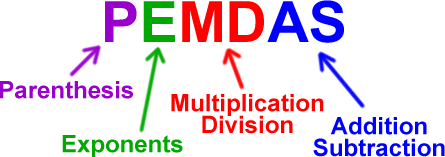
which is abbreviated by PEMDAS.

The P in PEMDAS stands for "parenthesis"

Parenthesis in math are used to group important things together, so you always do them first. 

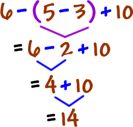
For example: 

 Do inside the parenthesis first:

Here's another Example: 

 In this problem we have to do paranthesis first then exponents then division.

The classic sentence that math geeks have been using for years to remember the Order of Operations (PEMDAS) is: 

Please Excuse My Dear Aunt Sally

Can you think of a sentence to go along with this acronym?

Murder Mystery- Geometry Game

After a lesson on shapes, angles and measurements i will put my students to the  test with a fun interactive game called Murder Mystery. This game will get the students up out of their seats to find clues and find who the suspect is. This game is kind of like the board game clue, students have to search through clues to find the murder.

Geometry Game- Murder Mystery: 

The Scene: The police are called to a high school, lying on the floor in the library is a dead student. As police search the library they find 5 clues written down by witness. They have sent the clues to you to decipher. They also provide a list of those present at the time of the murder. (This list is all the students in the class,  with specific details on each of the students). There are 32 suspects, each clue will eliminate half the number of suspects remaining. When all clues have been solved the suspected person will be revealed. 

Clue One: Get into Shape:

The answer to each number is a letter A=1, B=2, etc. 

1. Total number of sides of all four squares.

2. An octagon has ? sides. 

3. A square based pyramid has ? vertices. 

4. A pentagon has ? sides. 

5. A parallelogram has ? sides.

There are many more questions about 20 but I'm just giving you an example of questions you can ask. 

Clue Two: Look From a New Angle: 

I will provide the students with different kinds of angles and they will have to figure out the angle measure of each line. By the same system as above a = 10 degree, b = 20 degrees, and so on. 

For example: 

The rest of the clues also have to do with things the students learned from this particular lesson, they will have a clue on compass/directions, and also coordinating points on a plane. The last clue i will give them a story and they will have to find the error that is wrong in that story to find the suspect. 

I got this idea from another teacher but put my own spin on it, I will use my actually students as the suspects and I will let them choose if they wanna work together or not. None of the students will know who the suspect is until the game is over. This gets them up and moving around and also has them use their ipad's for clue number two. The story I also provide them with will also be available on their ipad's so they can see if they can spot what doesn't belong in the story. I have never done this game before but am looking forward to trying it in my classroom one day. I think this game can be for any grade and for any subject. The teacher just needs to have fun creating the questions, and the students need to have fun trying to figure out the clues. 

Welcome to my Technology Mathematical Educational Blog

This is a blog that I have already created to enhance students knowledge about specific topics in Discrete Mathematics (also know as Calc 4). I will be incorporating technology into my classroom also so many of my posts will be ways to incorporate technology into the mathematical classroom. I will be sharing different lesson plans, activities and my thoughts on certain math topics. Can't wait to hear feedback from my fellow classmates about incorporating technology into the classroom. At the rate technology keeps improving, we as teachers need to find new ways to keep up with the students and make learning more interesting to them. 

Graph Coloring

Graph Coloring: 

In Graph Theory, graph coloring is a special case of graph labeling. It is an assignment of labels traditionally called "colors" to elements of a graph subject to certain constraints. In the easiest form it is a way of coloring the vertices of a graph so that no two adjacent vertices share the same color, this is called vertex coloring. An edge coloring assigns a color to each edge so that no two adjacent edges share the same color, and a face coloring of a planar graph assigns a color to each face or region so that no two faces that share a boundary have the same color. 

A proper vertex coloring of the Petersen graph with three colors

The convention of using colors originates from coloring the countries of a map, where each face is literally covered. By planar duality it became coloring the vertices, and in this form it generalizes to all graphs. For example: In mathematical and computer representations, it is typical to use the first few positive or nonnegative integers as the colors. In general we can use any finite set as the "color set." Graph coloring enjoys many practical applications as well as theoretical challenges. Beside the classical types of problems, different limitations can also be set on the graph, or on the way a color is assigned, or even on the color itself. It has even reached popularity with the public in the form of the popular number game Sudoku. 

There are twelve different ways to color the map from above using three colors. 

A coloring using at most k colors is called k-coloring. The smallest number of colors needed to color a graph G is called its chromatic number, and is often denoted X(G) or Y(G). The chromatic number of a graph G is the smallest number of colors needed to color the vertices of G so that no two adjacent vertices share the same color. 

Examples: 

Examine Questions: Find the chromatic number for each graph listed below?  

Citations: Wikipedia, and Google images

Stable Marriages

The stable marriage problem is another classic appreciation of discrete mathematics to social networks. 

Suppose that you have been hired to be a matchmaker with n men and n woman who wish to be paired up with their perfect matches. Each man provides the matchmaker with a list of the woman ranking from first choice to last choice, as same for the woman. 

The matchmakers job is to provide a way to pair up the n men and n women in such a way so no man or woman is left behind. 

The stable marriage theorem states that your job can always be accomplished, no matter how the men and women have ranked one another. This theorem provides an algorithm that accomplishes your task. 

In round 1: every man proposes to his first choice. those woman who receives the offers tentatively accept the best offer and tell the other men not to come back. The rejected men then propose to their next choice, and the women then tentatively accept the best offer they have so far received and tell the other proposers to go away. This process continues until every man and woman are paired up. 

Example One: Suppose the matchmaker receives the following list: 

man 1 (3,1,4,2,5)

man 2 (1,3,5,2,4) 

man 3 (5,4,3,2,1)

man 4 (1,5,4,2,3)

man 5 (3.4.5.1.2)

woman 1 (3,5,1,4,2) 

woman 2 (3,1,2,4,5)

woman 3 (1,2,3,4,5)

woman 4 (5,3,1,2,4)

woman 5 (5,4,3,2,1)

 Use the stable marriage algorithm to find a stable parring. 

Answer: Men 1,2,3,4 and 5 will propose to women 3,1,5, 1, and 3 respectively. Woman 1 rejects man 2, woman 3 rejects man 5. So then men 2 and 5 propose to women 3 and 4 respectively, but man 2 is rejected again because woman 3 is already taken. Man 2 now continues to move down his list to woman number 5, who accepts him and rejects man number 3. Now man 3 proposes to woman 3, who rejects him. Then man 3 proposes to woman 2 who accepts his offer. WIth no man or woman unattached, the algorithm terminates with stable pairings: 

man 1 with woman 3, man 2 with woman 5, man 3 with woman 2, man 4 with woman 1, and man 5 with woman 4. 

Examine Question: Suppose the matchmaker receives the following list: 

man 1 (c, a, d, b, e)

man 2 (a, c, e, b, d) 

man 3 (e, d, c, b, a) 

man 4 (a, e, d, c, b)

man 5 (c, d, e, b, a)

woman a (3,1,2,4,5)

woman b (3, 5, 1, 4, 2)

woman c (5,3,1,2,4)

woman d (1,2,3,4,5)

woman e (5,4,3,2,1)

A. Use the stable marriage algorithm to find a solution pairing. (men proposes to women)

B. Find another stable marriage obtained by having the women propose to the men. 

RSA Method of Cryptography

RSA: is a crypt o-system, which is known as one of the first practicable public-key crypt o-systems and is widely used for secured data transmission. This method was named after three mathematically trained computer sciences, Ronald Riverst, Aid Shamer, and Lenorad Adleman, who discovered this method in 1977.

In the crypt o-system the encryption key is public and differs from the decryption key which is kept a secret. 

How it works: The bank publishes two numbers on its website, n and e (as in encipher), n and e are about 2000 digits long. 

1, Write your plain text should be under 1000 characters

for example: quiz today   

2. Convert your plain text to a number m (under 2000 digits) by replacing each letter with its 2-digit position in the alphabet

for example: 172109262015040125

3. Computer cipher text C=M raised to the e power mod n. Your the one emailing the C to the bank. 

4. When the bank receives your C, it uses a magic secret number d ( as its decipher) and computes C raised to the d mod n, which equals M. Then it converts M back to your plain text. 

The Encryption: An example of this is: if Brittany transmits her public key (n,e) to Billy and keeps the private key secret. Billy then wishes to send message M to Brittany. He first turns M into an integer m, such that 0 ≤ m < n by using an agreed protocol of the system. he then computes the cipher text c 

corresponding to , then Billy transmits c to Alice. 

The Decryption: Brittany can recover m from c by using her private key exponent d from the formula 

. Given m, she can recover the original message M.

Example One: Compute the following RSA method where p=5 and q=29. Find e and f, and also d to figure out what the value of M will be? 

To find the value of n we multiply p by q. 

so since p=5 and q=29 so (p)(q)=145. 

Now we need to find (n)

(145) = 4 x 28 = 112

We pick d=3 and then find e and f so that 

ed + (n) f =1

3 e + 112 f  =1

3(-37) + 112(1) =1

so e = -37

Now we send the message to M=2. 

The sent message is 

.

Exam Question: Compute the following RSA method where p=3 and q =7. Find e, f. and d to figure out what value M with encryption and decryption? 

Citations: Wikipedia and Our Math notes 

The Chinese Remainder Theorem:

The Chinese Remainder Theorem: is a result of congruences in number theory and some aspects of abstract algebra. It was first published in the 3rd to 5th centuries by Chinese mathematician Sun Tzu. 

The Chinese Remainder Theorem: says if m (one) and m (two) are relatively prime then the system of congruences 

has a unique solution mod m (one) m (two). 

"max" + "may"= 

Example: Find the unique solution to the following congruences: 

so, now we assign all the letters to a specific number,

since (11,9) =1, then there exists x and y so that 

11x+9y=1

using Euclid's formula: we see that 11(5) + 9(-6) = 1

so by this formula we see that x=5 and y= -6. 

Now we will use the "max" + "may" formula: 

=11(2)(5)+ 9(6)(-6)

=  110 - 324

= -214

therefore N=83. 

Example: Find the unique solution to the following congruences: 

so now we assign the letters to a specific number, 

since (5,3) =1 then there exists x and y so that

5x + 3y =1

using Euclid's formula: we see that 5(2) + 3(-3) =1

so by this formula we see that x=2 and y=-3. 

Now we will use the "max"+ " may" formula: 

= 5(2)(2) + 3(3)(-3)

= 20 + -27

= -7

therefore N = 8

Quiz Question: Find the unique solution to the following congruences: 

using the chinese remainder theorem and the "max" + "min" formula. 

.

Credit due to: wikipedia and my class notes

Modular Arithmetic

MODULAR ARITHMETIC: 

Modular Arithmetic is the mathematics of remainders. 

 if m l a-b the number m is called the modulus. 

A common example for Modular Arithmetic is Clock Arithmetic: 

There is an additive law to modular arithmetic that says: 

There is also a commutative law to modular arithmetic that says: 

Example: What is 38 mod 12?

So what you do is divide 12 into 38 and see what the remainder is, 

Example: What is 59 mod 4? 

Examine Question: What is 83 mod 5? 

There are two different tricks to finding mod's the first method is called the casting out nines method: 

the casting out nines method states that for a positive integer x, we define S(x) to be the sum of the digits of x. 

Example: What is S(5409)?

So we need to add all the number in S(x) together and we get 5+4+0+9=18

Now we claim: that 

so using our claim we get 

Examine Question: What is S(1688)?

The second method is just like the casting out of the nines method but using mod 11. So for a positive integer x, we define S(x) to sum of the digits of x. 

Example: What is S(13748)? 

1-3+7-4+8=13

Now we claim that

so using our claim we get 

Examine Question: What is S(34693)?

Work cited to: our lecture notes